This article is part of our series on Delimitation of hydrographic sub-basins using QGIS and a DEM:
- Delimitation of hydrographic sub-basins using QGIS and a DEM
- Digital elevation models for hydrological studies
- Technical criteria for the delimitation of sub-basins
- Sub-basin delimitation process using QGIS (This post)
In this article we are going to explain the process to delimit the river sub-basins of a certain region using QGIS and a DEM. In this case the region is the entire Republic of Mozambique.
The starting data we need is a mosaic of Digital Elevation Models (DEMs) of the entire area and the watershed layer. As we commented in the previous articles of the series, we will use the NASADEM HGT mosaics (here we explain how to download them) and the basin layer elaborated by GEAMA.
Create single DEM (Mosaic)
The first step is the union of the DEM mosaics to create a single DEM for all of Mozambique.
QGIS provides us with different options for joining raster files. In this case we are going to use the tool “Merge”. To do this, select “Raster” from the menu, display the “Miscellaneous” options and click “Merge”.
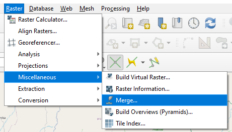
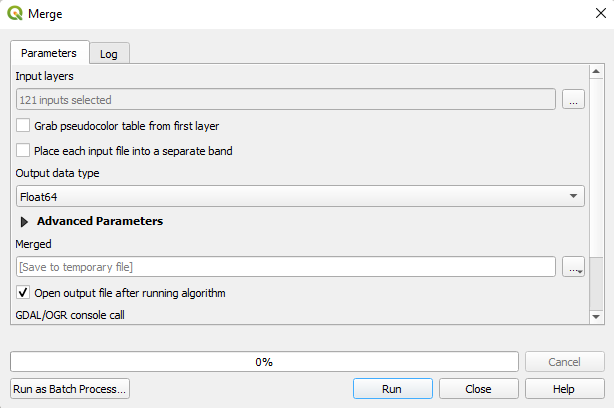
In the pop-up window we add all the input layers, that is, all the DEMs downloaded from the web of the area in which we are going to work. We give a path and a name for the output file, check the option “Open the output file after running the algorithm” and execute.
DEM reprojection
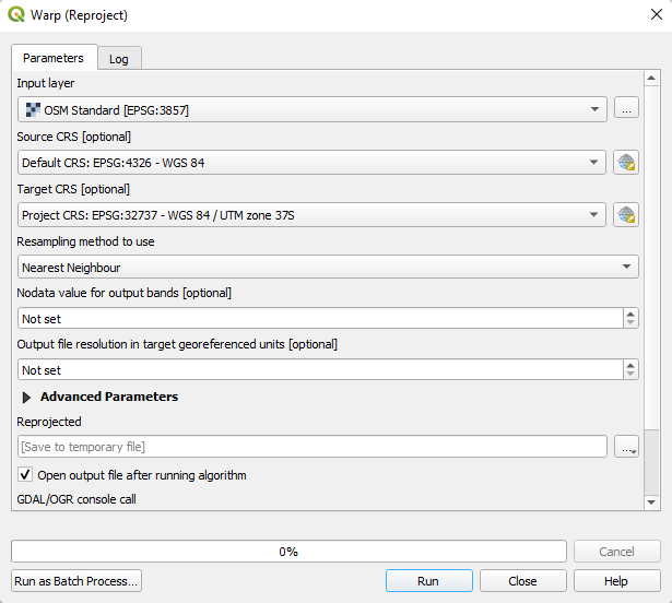
The merged DEM is in the WGS 84 Geographic Coordinate System (EPSG:4326). We reproject the DEM to a Projected Coordinate System. In our case to WGS 84 / UTM zone 37S (EPSG:32737). To reproject the DEM from the menu we select “Raster”, then “Projections” and “Warp (reproject)”.
In the input layer we select the combined DEM and indicate both the source CRS and the target CRS. We also indicate a path and a name for the output file and run the algorithm.
DEM clipping
To reduce the processing computation of the algorithms that we will use in the following steps, we will now clip the DEM per each river basin. Another reason for making these cuts is the difference in sizes and shapes of the basins that we are going to analyze. Better results will be obtained by analyzing each basin separately in order to adjust the parameters of the algorithms to each particular case instead of using the same parameters for all of Mozambique.
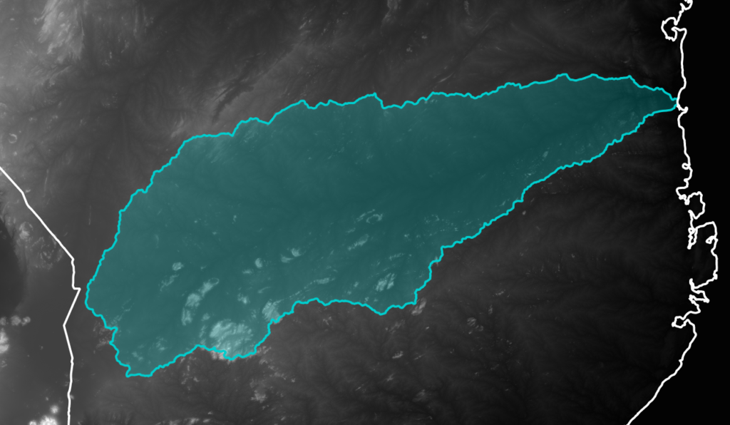
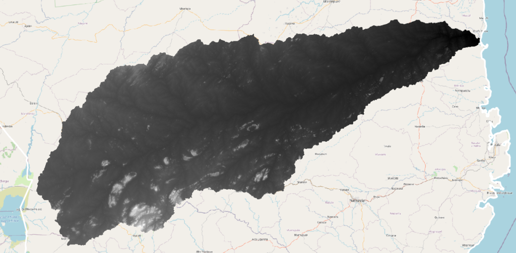
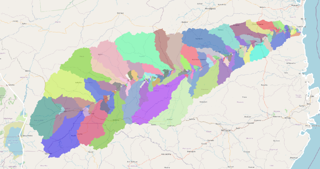
We create the masks for each basin from the basins layer. In the following image you can see the DEM in the background, in white the administrative limit of Mozambique and in blue the mask of the Lurio river basin.
Next, we clip the DEM with each created mask. To clip the DEM, in the main menu we select “Raster”, then “Extraction” and “Clip Raster by Mask Layer”.
In the pop-up window we select the reprojected DEM on the input layer and the basin mask on the mask layer. Also, so that the crop fits exactly to the edge of the basin and so that no black area is visible, we will specify a value for “no data”, for example -9999. Finally, we mark the following two options:
- Match the extent of the clipped raster to the extent of the mask layer.
- Keep resolution of input raster.
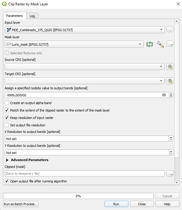
We specify the path and name for the output file and run the algorithm.
Perform this process for all basins. Batch processing can be used for this instead of doing it one by one.
Filling depressions
Although the latest versions of the DEMs are already processed with different corrections and gap filling, they may still contain artifacts such as depressions. Artifacts must be removed before using a DEM in hydrologic analysis. There are several algorithms for filling gaps (GDAL, GRASS, SAGA, …). The incorporation of the GRASS hydrological toolset in QGIS is very useful. We will therefore use the GRASS algorithm both for this step and for others that we will see later.
To fill depressions we wil use the processing toolboox, if it is not visible on the right side of the QGIS window, it can be enabled from the main menu, by select “Processing” and “Toolbox”.
In the toolbox find or type the following algorithm: r.fill.dir. In the dialog window select as input (Elevation) the clipped DEM and uncheck Flow direction and Problem areas. We are only interested in obtaining the DEM without depressions. Indicate the path and name for the output file and execute.
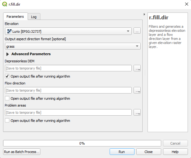
This geoprocess can take a long time to finish depending on the size of the raster and the power of the computer. Perform this geoprocess for all basins. Batch processing can be used for this instead of doing it one by one.
Drainage direction, accumulated flow, stream segments and sub-basins
Now that we have a corrected DEM, the next step is to calculate the drainage directions, accumulated flow, stream segments and sub-basins. To do this we look for the following algorithm in the toolbox: r.watershed
In the dialog window we select the corrected raster of the basin and establish the most appropriate “Minimum size of exterior watershed basin” for each case.
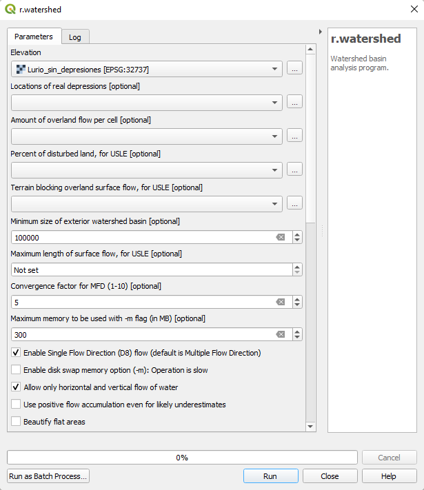
Because of the wide difference between the size of some basins and others, it is necessary to play with the “Minimum size of exterior watershed basin” to obtain the optimal results for each of them.
An average size can be obtained by reviewing the characteristics of the raster. The pixel size of the raster is 30x30m, so the “Minimum size of exterior watershed basin” must be at least 333,333.33 pixels, approximating 300,000 pixels.
But, in many cases, it is decided to establish 100,000 or less to solve some problems detected in some flat areas or mouths. Also check the following two options:
- Enable Single Flow Direction (D8) flow
- Allow only horizontal and vertical flow of water
Also check the boxes that can be seen in the following image, in addition to indicating the paths and names of the output files and execute the algorithm.
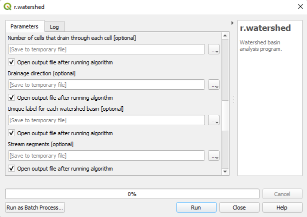
We thus obtain for each basin:
- Accumulated flow
- Drainage direction
- Sub-basins
- Stream segments
The only layer we are going to work on is the sub-basin layer, the rest are calculated to serve as support for small manual adjustments that we will make later.
Transform to vector layer
Once we have the sub-basins layer, the next step is to transform this raster layer into a vector layer. To do this we are going to look for the following geoprocess in the toolbox: r.to.vect. In the window, select the sub-basins layer as the input raster layer.
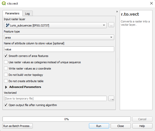
Also select these options and run:
- Feature type: area
- Smooth corners of area features
- v.out.ogr output type: area
Review and manual adjustments
Once we have the vector layer of sub-basins we have to review the result, join the necessary polygons to have only the sub-basins that meet the agreed criteria mentioned in the previous article and make small manual corrections where necessary.
The union of the polygons is also necessary because the algorithm creates sub-basins of tributaries that are not direct to the main river, that is, tributaries of a tributary of the main river. In this way we solve the problem.
These algorithms work well in sloping areas, but in flat areas they can give undesirable results, and it is necessary to review them. For example, in coastal areas with very flat basins, a more detailed review and adjustments to sub-basin boundaries were required based on other information such as drainage directions, rivers, etc.
Smoothing and simplification
When vectorizing a raster, the edges of the polygons are generated following the shape of the pixels, for this reason it is necessary to smooth them.
This leads to another problem, which is that smoothing creates many vertices that make the layer size increase quite a bit. To avoid this, after smoothing you can also do a simplification.
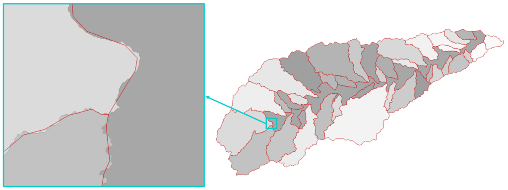
Choosing the appropriate parameters, smoothing and simplification are carried out without practically losing definition in the delimitation of the sub-basins. In the image below you can see the edges of the sub-basins before and after (red) smoothing and simplifying.
Sub-basins merge
Since we have created a sub-basin layer for each basin, we perform a vector layer union to create a single sub-basin layer for the entire country: mergevectorlayers.
In the dialog window we select all the sub-basin layers for input layers, we specify the Coordinate Reference System, the path and the name of the output file and we execute.
Geometric and topological checks and corrections
Once we have the desired sub-basin layer, overlaps, duplicates, gaps, invalid geometries, etc. must be checked and corrected.
This can be done with plugins (Manage and install plugins)
Modify attribute table as needed
In addition to the geometry of the sub-basins, we must also add the desired attributes and order the attribute table as desired. Some examples of useful attributes in a sub-basin layer are the name of the river, the area, length of the main river or the basin to which it belongs.
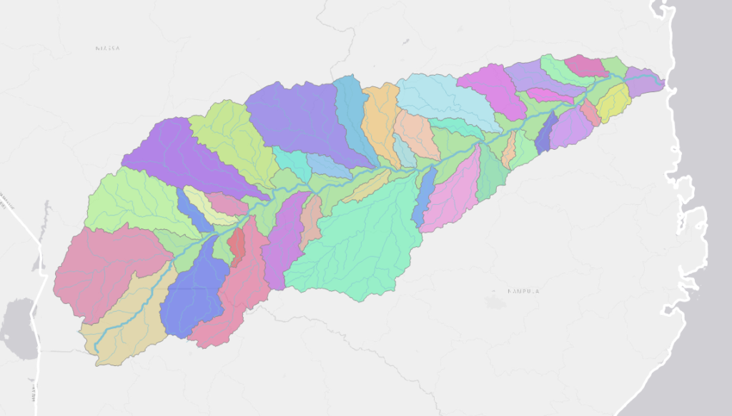
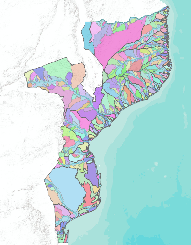
Final Results
Following these steps we obtain our layer of sub-basins.
With this article we close our series on the delimitation of sub-basins. Did you find them interesting? Do you use other techniques? Need help? Get in touch with us or write to us on Twitter.